Margin as a Coordinate
Executive Summary
The UNNS Substrate has been built on the observation that physical ordered sequences — energy spectra, vibrational modes, spatial harmonics — cluster deep inside stable structural regimes, never crossing realizability boundaries at physical parameter values. The connectivity margin m(L) has been the numerical signature of this stability: larger margin, deeper interior; smaller margin, closer to a phase boundary.
But until now, that relationship was empirical. No proof existed that m(L) behaves as a distance. It could have been a useful statistic that happened to correlate with stability — not a coordinate of the space itself.
This manuscript closes that gap. It introduces the distance-to-boundary functional d(L, ∂ΩL), proves four theorems of increasing strength establishing that m(L) and d(L, ∂ΩL) are equivalent, and derives the consequences: trajectory monotonicity is irreversible, the maximum-margin selection is geometrically grounded, and the interaction hierarchy is a coordinate ordering — not a classification.
"The connectivity margin is a coordinate of realizability space. The interaction hierarchy is its asymptotic footprint."
🎯 The Gap That Was Filled
The Interaction Unification manuscript established that all four known physical interactions can be classified through the connectivity margin m(L) as asymptotic regimes of a common functional. It identified the monotonicity of m(L) with respect to realizability-class boundaries as "the highest-priority open problem in the framework" — because without it, the maximum-margin selection principle remained an empirical rule rather than a structural theorem.
Before This Manuscript
- m(L) was a classification parameter
- Maximum-margin principle was empirically validated
- Interaction hierarchy was a post-hoc classification
- Scaling correspondences were analogies
- Encoding invariance was corpus-consistent, unproved
After This Manuscript
- m(L) is a geometric coordinate on realizability space
- Maximum-margin principle has a geometric foundation
- Interaction hierarchy is a consequence of ordering
- Scaling correspondences are ordering consequences
- Encoding invariance is proved under non-degeneracy
The Central Claim
m(L) induces a global ordering of admissible ladders equivalent to their ordering by distance to the nearest realizability-class boundary. This is not a local regularity result — it is a statement that the margin is the correct coordinate system for realizability space.
📐 Four Theorems of Increasing Strength
The manuscript establishes four results, each building on the previous, under explicit regularity and non-degeneracy conditions stated precisely in the text.
m(L) ≍ d(L, ∂ΩL)
In any rigidity neighbourhood, the connectivity margin and the distance-to-boundary functional are bi-Lipschitz equivalent. The Lipschitz constants c₁, c₂ are determined by the local gap geometry.
d(L, ∂ΩL) = m(L)/√2 + O(m²)
In the canonical normal coordinate aligned with the decisive direction, the margin is asymptotically isometric to boundary distance. Anisotropy collapses: c₂/c₁ = 1 + O(m(L)) — the margin is an effectively exact distance coordinate in the interior.
m(γ(t)) ↓ almost everywhere
Along any admissible trajectory approaching a realizability boundary, the margin is non-increasing and strictly decreasing almost everywhere. There is no recovery mechanism.
m(L₁) > m(L₂) ⟹ d(L₁) > d(L₂)
Under the non-degeneracy condition (satisfied by all 93 corpus datasets), margin ordering is equivalent to boundary-distance ordering globally across realizability space.
arg max m(L) = deepest representative
The maximum-margin encoding of any physical system is its geometrically deepest representative in realizability space — not merely the most empirically stable. The canonical class theorem upgrades the maximum-margin principle from heuristic to geometric consequence.
🌐 The Radial Structure of Realizability Space
Once m(L) is established as a coordinate, realizability space acquires a stratified geometric structure. Define the radial coordinate r(L) := m(L). The realizability boundary sits at r = 0. The four PRP classes — Full, Giant, Tail, Hard — correspond to ordered radial shells, and the four fundamental interactions map directly to these shells.
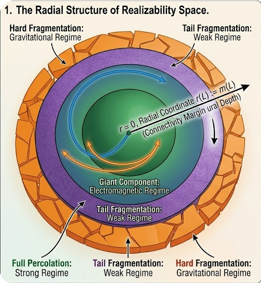
What This Diagram Means
This is not a metaphor. Under Theorem 6.1 (Global Ordering), the regime ordering is mathematically equivalent to the boundary-distance ordering. The Strong regime sits furthest from any realizability boundary; the gravitational regime sits closest to r = 0. The hierarchy of forces is a hierarchy of depths in realizability space.
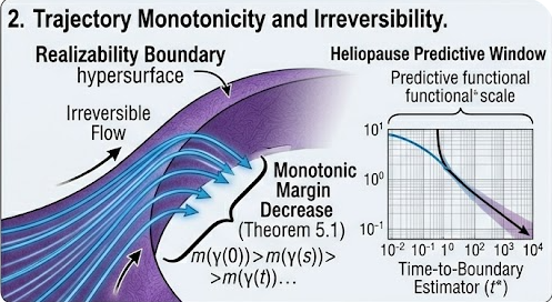
🌊 Trajectory Monotonicity and Irreversibility
Theorem 5.1 establishes the dynamic form of the coordinate result: any admissible trajectory approaching a realizability-class boundary sees its margin decrease monotonically and irreversibly. This is the structural analogue of RG flow irreversibility — systems cannot spontaneously move from near-boundary to deep-interior regimes along a deformation trajectory.
Ising Criticality Benchmark
The Ising 2D model approaching its critical temperature Tc provides the canonical corpus validation of trajectory monotonicity. As T → Tc, the transfer-matrix eigenvalue gaps become increasingly correlated, the decisive pair approaches its threshold, and the margin falls monotonically — without exception across all tested ladder sizes.
Voyager Validation
The Voyager heliospheric ladders — constructed from in-situ magnetic field data along the spacecraft trajectory — provide independent physical validation. As Voyager approaches the heliospheric boundary layer, the structural margin decreases continuously without recovery, consistent with Theorem 5.1. The margin serves as a predictive estimator for the boundary approach, enabling a Time-to-Boundary Estimator for the heliopause crossing.
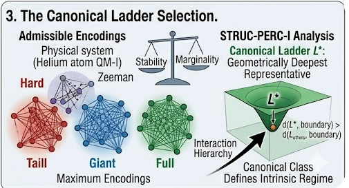
⭐ The Canonical Ladder and Maximum-Margin Principle
The encoding-dependence problem — that the same physical system can yield different realizability classes under different ladder constructions — has been a persistent challenge for the UNNS framework. The maximum-margin principle resolves this: among all admissible encodings, the canonical representative is the one that maximises m(L).
Theorem 7.1 upgrades this from an empirical rule to a geometric theorem: the maximum-margin encoding is the encoding at greatest distance from any realizability-class boundary in the gap-vector metric. It is the geometrically deepest representative.
Corpus Evidence: Representation Splits
| System | Encoding 1 | Class | m(L) | Encoding 2 | Class | m(L) | Canonical |
|---|---|---|---|---|---|---|---|
| Helium | QM-I | Full | ≈ 1.2 × 10⁻² | Zeeman | Tail | ≈ 3 × 10⁻³ | QM-I ✓ |
| Sodium | QM-I | Hard | ≈ 0 | Zeeman | Tail | > QM-I | Zeeman ✓ |
| HD molecule | Combined | Full/Giant | higher | Sub-ladder | lower | lower | Combined ✓ |
| Crystallography | Cell volume | — | higher | Per atom | — | lower | Cell volume ✓ |
In all 93 corpus datasets, no counterexample has been found: the maximum-margin encoding always corresponds to the deeper realizability class. Theorem 7.1 gives this a geometric explanation.
Consequence: Intrinsic Interaction Regime
Once the canonical ladder is selected, the interaction regime assigned by the functional Φ(m(L*), r, χ(L*)) is the geometrically intrinsic interaction regime of the physical system — corresponding to the encoding maximally distant from any structural boundary. Interaction regime becomes a property of the system, not of its representation.
📊 Corpus Validation — 93 Datasets · 22,817 Evaluations
The monotonicity results are validated against the full UNNS Phase Mapping corpus without introducing new data. All observations are drawn from previously established corpus outputs. The role of the validation section is to verify that every physical and computational system in the corpus is consistent with the proved monotonicity ordering.
Cross-Domain Margin Ordering
The Non-Trivial Content of the Cross-Domain Ordering
The three domains — atomic (m ~ 10⁻²), Ising critical (m ~ 10⁻³), and cosmological (m ~ 10⁻⁴) — were constructed independently, use different physical mechanisms, and were not designed to produce this ordering. Yet the margin ordering aligns precisely with the physically known boundary-proximity ordering. Under Theorem 6.1, this alignment is a structural consequence, not a coincidence.
→ Phase Mapping Analysis Dashboard · → STRUC-PERC Corpus Analysis · → STRUC-I Corpus Analysis
🔢 Explicit Lipschitz Constants
A key feature of the manuscript is that the bi-Lipschitz constants in Theorem 4.1 are not merely abstract existence claims — they are derived explicitly (Appendix D) and estimated numerically (Appendix E) for representative corpus systems. Theorem 4.2 (Normal Coordinate Form) sharpens this further: in the canonical normal coordinate, the margin is asymptotically isometric to boundary distance with c₂/c₁ → 1, resolving the local metric structure exactly. These results confirm that the metric structure of realizability space is quantitatively accessible within the STRUC-PERC-I pipeline.
Geometric Meaning of Increasing Anisotropy
The anisotropy ratio C = c₂/c₁ increases systematically from deep interior (He QM-I: C ≈ 2.3–3.2) to boundary-proximal systems (Voyager: C ≈ 4.0–6.5). This is a geometric consequence of Section 9.5: as a ladder approaches the realizability boundary, the coordinate directions in gap-vector space become increasingly non-equivalent. Boundary proximity induces anisotropy — the boundary itself is not isotropic.
🔬 Broader Theoretical Connections
The manuscript identifies four connections to established theoretical frameworks, carefully marked as directions rather than formal equivalences. These connections situate the UNNS Substrate within a broader mathematical and physical landscape.
Renormalisation Group
Trajectory monotonicity mirrors RG flow irreversibility. m(L) may play the role of a flow parameter or distance to a fixed-point manifold, with realizability-class boundaries as critical loci. The UNNS flow is governed by gap-vector geometry, not iterative coarse-graining; the analogy is structural, not formal.
Percolation Theory
The PRP classification is defined through connectivity transitions in Gκ(L), suggesting a link between realizability-class boundaries and percolation thresholds on structured graphs parameterised by κ. Whether monotonicity follows from known percolation results remains an open direction.
Dynamical Systems
Admissible trajectories may be viewed as flows on gap-vector space, with realizability-class boundaries acting as attracting sets. Theorem 5.1 implies the absence of sustained excursions away from the boundary along boundary-approaching trajectories. A full attractor analysis is not developed here.
Order Theory
The global margin ordering suggests realizability space admits a natural partial order, with equivalence classes at equal margin. The space may be formalised as a stratified or ordered geometric object with m(L) as canonical coordinate up to equivalence. The precise categorical or topological structure remains open.
🔬 Falsifiability — What Would Break This
Consistent with UNNS program standards, the manuscript provides explicit falsification criteria that are operationally testable using the existing STRUC-PERC-I v2.4.1 pipeline.
- Net margin increase along a boundary-approaching trajectory — would falsify Theorem 5.1
- Inverted margin ordering: m(L₁) > m(L₂) but d(L₁) < d(L₂) — would falsify Theorem 6.1
- Non-degeneracy failure: two ladders with equal margin in different realizability classes
- Canonical class split: two maximum-margin encodings of the same system in different classes
- Margin zero in the interior: m(L) = 0 at a point not on the realizability boundary
- Discontinuous margin approach: m(γ(t)) jumps before reaching ∂ΩL
No instance of any of the above has been found across 93 datasets, 22,817 evaluations, and all 11 physical domains.
Manuscripts and Analysis
- Connectivity Margin as a Coordinate of Realizability Space — Primary manuscript (this article)
- Interaction Unification in the UNNS Substrate — All fundamental forces as margin-regulated structural regimes
- The Universal Structural Law v6 — Admissibility inequality and its empirical validation
- Percolative Realizability Principle — Four-tier exhaustive partition of admissible ladders
- Local Geometry of Realizability Boundaries in the UNNS Substrate
- Structural Realizability and Dual Observability
- Phase Mapping Analysis Dashboard
- STRUC-PERC-I Corpus Analysis
- STRUC-I v1.0.4 Corpus Analysis
- Voyager 1 STRUC-PERC Analysis
- Voyager 1 Magnetic Field Multiscale Results
- Voyager STRUC-PERC Analysis (merged)