Voyager Reveals a Structural Boundary
in the Heliosphere
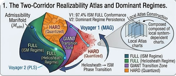
Where this happens — the realizability manifold
Every physical measurement can be sorted into a structural sequence — a ladder. The UNNS Substrate provides a formal geometric space, the admissibility manifold ℳadm, where all such ladders live. Different physical regimes occupy different regions of this space.
When a system evolves in time, it traces a path through ℳadm — a structural trajectory. Physical boundaries between regimes appear as geometric boundaries in ℳadm, and those boundaries leave measurable signatures in the data.
What ℳadm means in plain terms
Think of it as a map of structural states. Every physical observable, at every moment, maps to a point on this map. Different regimes cluster in different regions. A boundary crossing means moving from one region to another — and that movement has a geometric signature detectable from the data alone, regardless of what is being measured.
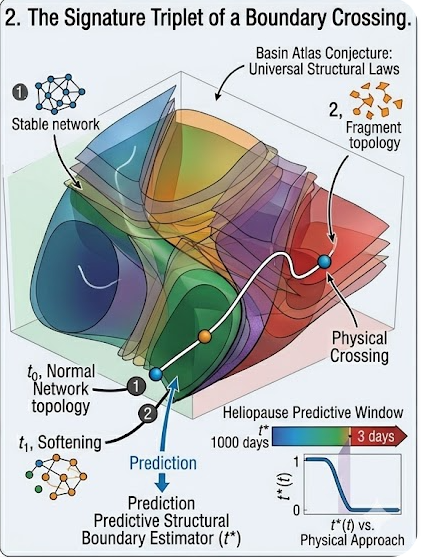
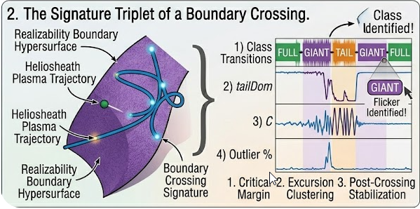
What a structural transition actually looks like
When a physical system approaches a realizability boundary, three things happen in sequence — predictably, regardless of domain. Together they form the Boundary Signature Triplet:
This triplet appears wherever a boundary crossing exists and is absent in control trajectories without a physical transition. It is diagnostic, not generic — which means it can serve as the basis for a formal detection operator.
Returns the boundary epoch from structural connectivity alone. Returns undefined when no boundary is detected — it does not always produce output.
The critical property
The operator is not fitted to data. Its admissibility conditions are fully specified before any data is seen and applied identically across all datasets. The result t* = 2012 follows from the Voyager data — not from tuning the method to match it.
📘 Formal foundation
The complete theoretical framework — including six conditional theorems, the Structural Boundary Operator, and the full multi-scale robustness analysis — is developed in the primary manuscript.
Read the full manuscript →What this looks like in real Voyager data
Voyager 1 crossed the heliopause in August 2012. The 48-second MAG dataset spans 2011–2017, covering heliosheath approach, crossing epoch, and five years of interstellar medium. 3,500 STRUC-PERC-I evaluations (500 windows per annual epoch) produce a structural trajectory of the magnetic field magnitude |B| through ℳadm.
Before and after — the physical validation
Voyager 2 (plasma data, 2007–2018) approached the heliopause but never crossed it in this dataset. Voyager 1 (magnetic field, 2011–2017) crossed it and recorded five years of post-crossing ISM. The two trajectories are not redundant — they are complementary projections of the same boundary object in ℳadm.
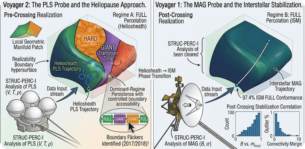
Two-trajectory structural tomography
Voyager 2 resolves the approach side: pre-heliopause softening, FULL→GIANT onset in 2017–2018. Voyager 1 resolves the crossing and post-crossing ISM basin. Together they reconstruct the heliopause boundary from two independent structural perspectives — the first two-sided geometric reconstruction of any physical boundary in the UNNS programme.
Key Findings
First Structural Boundary Detection
The heliopause is detected at t* = 2012 from connectivity data alone — no physical label, no domain model, no prior knowledge of the crossing location.
Scale-Invariant Result
The same epoch is identified at window sizes 512, 1024, and 2048 samples. The ordering of κconn is preserved across a fourfold scale variation.
ISM as Distinct Structural Basin
Post-crossing κ ranges (27k–36k) are completely disjoint from pre-crossing ranges (14k–18k). No overlap at any tested scale.
Universal Boundary Triplet
The three-signal signature appears at every realized boundary and is absent in negative controls. Diagnostic, not generic.
Two-Trajectory Tomography
Voyager 2 (approach) and Voyager 1 (crossing + ISM) are complementary projections of the same heliopause boundary object in ℳadm.
Operator with Failure Modes
The operator is proved correct under regularity conditions and explicitly returns undefined when admissibility conditions fail — no spurious outputs.
Why this matters
Physical phase transitions have always been characterized by changes in measurable quantities: temperature, pressure, density. This work takes a different approach. It shows that phase transitions can be detected as geometric events in a structural space, without knowing which physical quantities change or where the boundary is.
- Excursions are not noise. GIANT and TAIL structural windows near the boundary are signals of geometric proximity. They cluster because the structure of ℳadm requires it.
- The ISM has a structural identity. Not just a physical location — it is a distinct, measurable basin in ℳadm, separated from the heliosheath by a geometric boundary.
- The approach generalizes. The same operator, applied identically, has been observed across atomic spectra, cosmological structure, and any domain once embedded in ℳadm.
What makes this result reliable
Scale robustness — all three window sizes confirm t* = 2012
| Scale | Window duration | κ minimum | t* = 2012? | Excursion peak | Basin separation |
|---|---|---|---|---|---|
| W = 512 | ~6.8 h | 5 872 | ✓ | ✓ 2011–12 | ✓ No overlap |
| W = 1024 | ~13.7 h · baseline | 14 686 | ✓ | ✓ 2011–12 | ✓ No overlap |
| W = 2048 | ~27.3 h | 47 562 | ✓ | ✓ 2011–12 | ✓ No overlap |
Why this eliminates the segmentation objection
Absolute κ values change with window size — expected and unimportant. The ordering of annual means does not change. The operator depends only on the ordering. Therefore t* = 2012 reflects an intrinsic property of the trajectory, not a property of how the data was segmented.
What this establishes
This result changes how phase transitions can be identified. The heliopause crossing is not inferred from physical interpretation, but detected directly from structural organization. A boundary in physics appears as a geometric event in ℳadm, and its location is recoverable from data alone.
- Boundary detection becomes algorithmic — the transition epoch is obtained from a pre-specified operator, not from post hoc interpretation.
- Structural signals replace heuristic indicators — connectivity minima and excursion clustering act as direct markers of boundary proximity.
- Regimes acquire geometric meaning — the heliosheath and ISM are not just physical regions, but distinct structural basins with non-overlapping coordinates.
- The method is falsifiable — if the signature triplet is absent, the operator returns no boundary.
The decisive test
Apply the Structural Boundary Operator to an independent dataset with a known phase transition and show that it returns the correct epoch without any modification. A single successful replication would establish boundary detection as a domain-independent structural procedure.
Resources & References
- Primary Manuscript: Structural Phase Transitions Along Physical Trajectories — UNNS Manuscript Series, 2026. Six conditional theorems, Structural Boundary Operator, multi-scale robustness proof, basin atlas, negative controls, falsifiability framework.
- Corpus Analysis: Voyager 1 STRUC-PERC-I Analysis Report — Full per-epoch statistics, class distributions, annual κ tables, 2011–2017.
-
Multi-Scale Robustness:
Multi-Scale Window Robustness Report
— Controlled W=512/1024/2048 sweep results.
↳ Robustness Table (CSV)
↳ Summary Metrics (CSV)
(Reproducibility data used for robustness validation)
- Instrument: STRUC-PERC-I v2.5.0 — Interactive structural evaluation chamber with batch mode.
- Data: mag_48s_2.zip — CDF files, ladder pipeline, STRUC-PERC-I batch outputs.
- Physical reference: Raw data — Voyager 1 heliopause crossing: August 2012 (Stone et al. 2019, Nature Astronomy). MAG dataset: NASA CDAWeb · hires1991_2030/primary/mag_48s.