Close to the Vacuum, Far in Energy

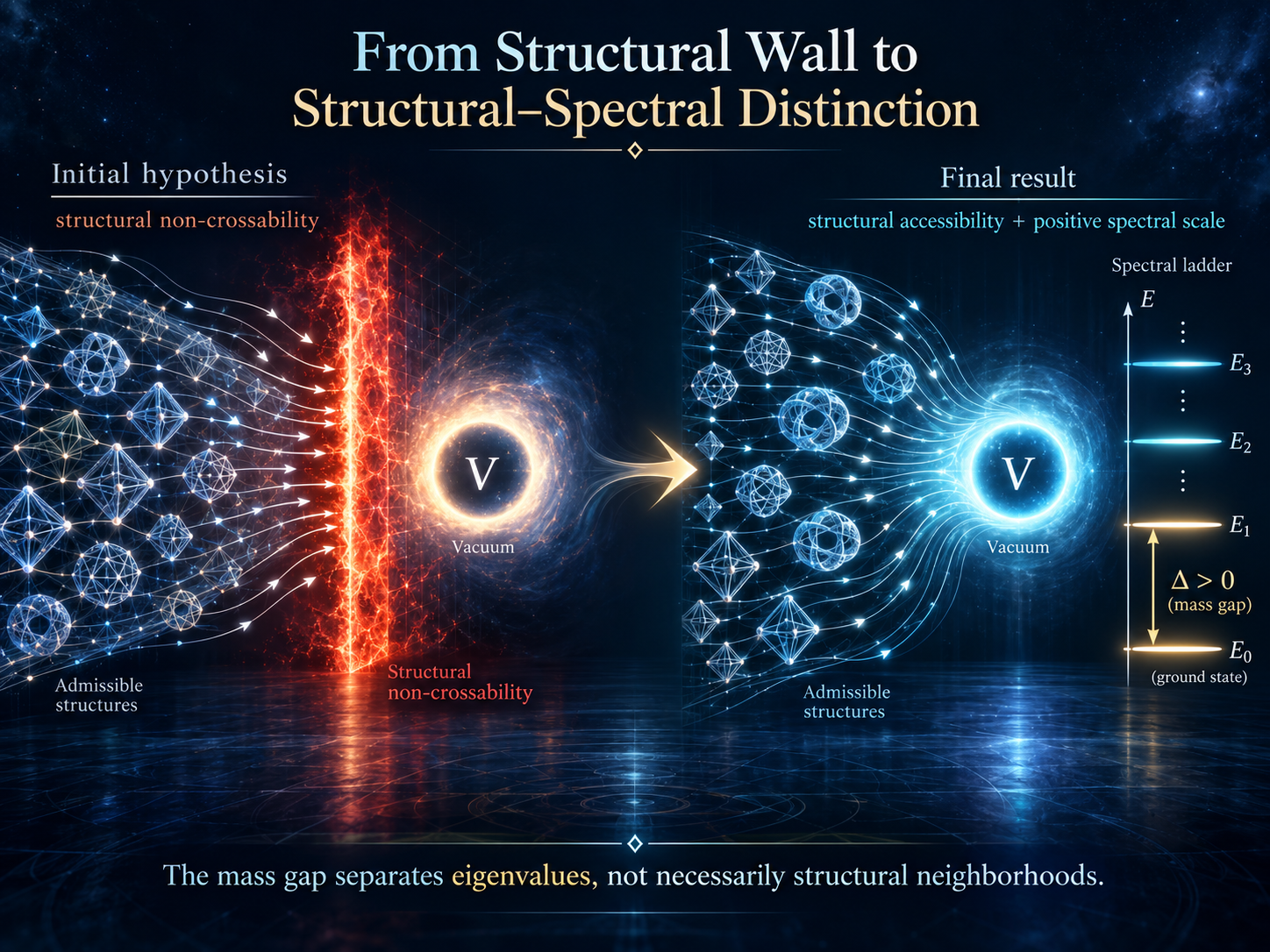
1We went looking for a wall

The question was deliberately strong. If it failed, it should fail visibly.

The idea was simple to state. Numerical pure-SU(3) lattice Yang–Mills spectroscopy exhibits a strictly positive lowest excitation scale. The open mathematical problem is whether the continuum quantum theory can be constructed with a rigorously positive mass gap. Perhaps that gap is not only a fact about energies. Perhaps it is written into the structure of the theory, so that the vacuum sits behind a refinement-stable exclusion boundary. Admissible, non-vacuum states would then never be able to come arbitrarily close to it, however finely we look.

That was the working hypothesis of the first project, UNNS_YM_GAP. It is an attractive picture, because it would turn an abstract spectral statement into something one could see: a gap in structural space.

The first project did not simply produce nothing. It built a diagnostic called CORR-I, showed that it separates massive from gapless controls at fixed resolution, and demonstrated model-level persistence under refinement, all before measured data became decisive.

The crucial question was whether the wall would survive contact with measured data.

2But what does “close to the vacuum” even mean?

Before following the data, there is a conceptual problem that the original hypothesis had hidden. “Close to the vacuum” sounds like one idea. It is at least four.

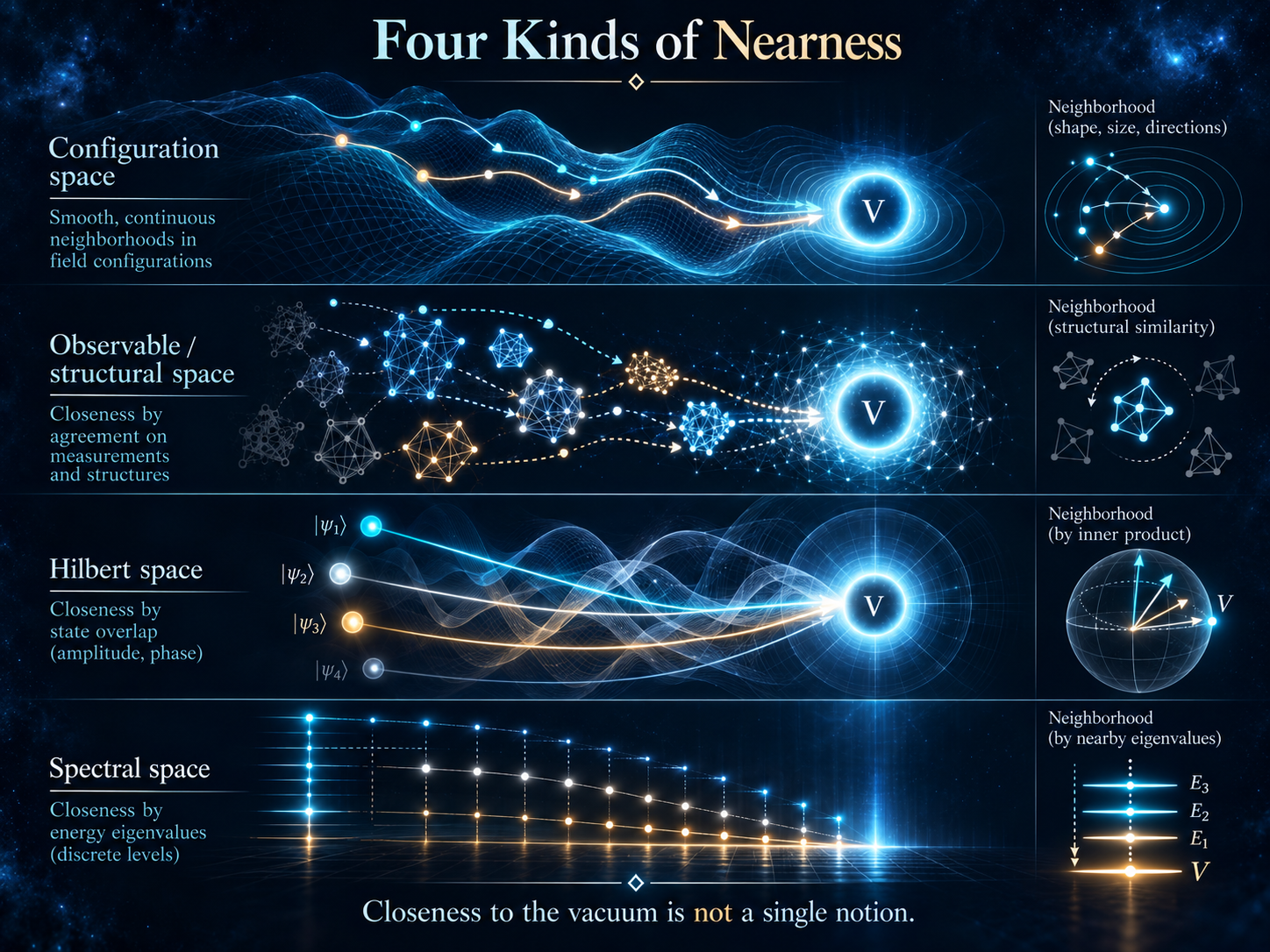
Figure 2 — Four kinds of nearness. “Close to the vacuum” is not a single mathematical notion. The synthesis distinguishes configuration-space, observable/structural, Hilbert-space, and spectral nearness. Nothing forces these four spaces to share the same topology, and the original structural-wall interpretation implicitly treated structural and spectral proximity as though they were equivalent.

These are not four names for the same distance. They live in different spaces, and nothing automatically forces their topologies to coincide. The original wall hypothesis quietly treated observable-space nearness as though it were spectral nearness. That distinction is one of the central conceptual gains of the research.

3Stage 1: the structural wall meets measured data

Now the first project, told properly. Its evidence came in two classes that were never allowed to blur together. Class C was a model branch: controlled refinement in which the diagnostic could be shown to behave as a wall picture predicts. Class B was the measured-data branch: a reconstruction from measured lattice data, where nothing is guaranteed to cooperate.

Class C behaved as expected. Eight refinement levels held the separation, and the frozen verdict was MODEL-REFINEMENT PERSISTENT. Class B did not.

Figure 3 — Stage 1 — testing the structural wall. The decisive measured-data challenge to universal non-crossability. Model controls retained refinement-stable separation, but the Class B reconstruction crossed the proposed boundary near β = 6.71, while its uncertainty interval still straddled zero. The correct frozen verdict was therefore DATA-INDETERMINATE: the structural-wall hypothesis was not established, rather than disproved or rescued by the model branch.

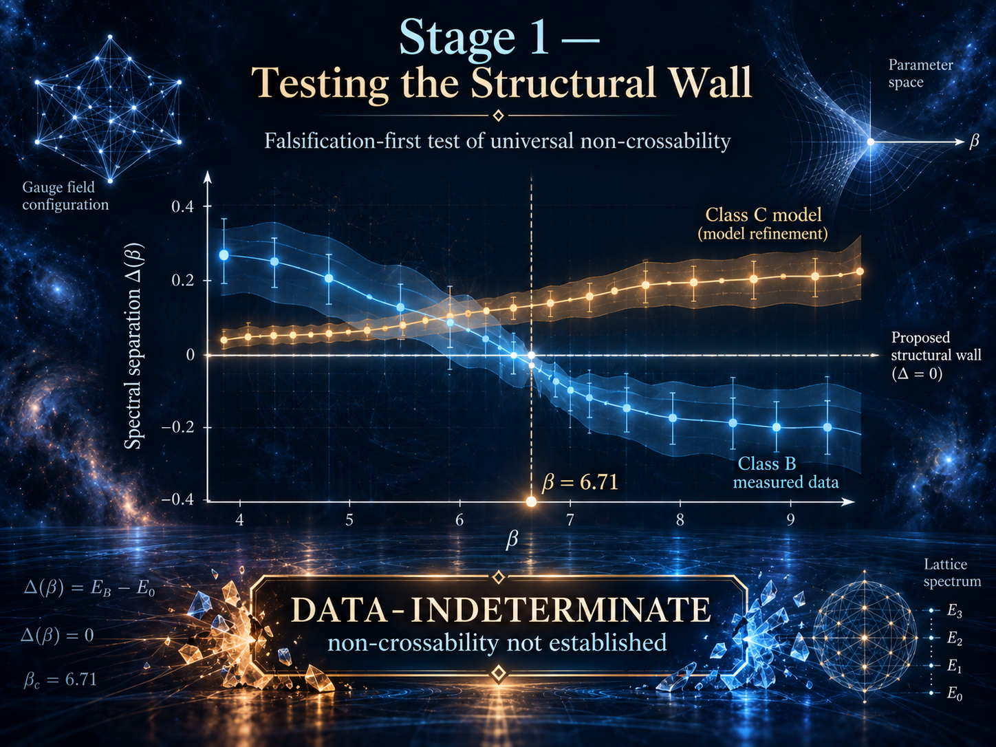
The numbers are small and honest. The Class B margin S_B stayed positive at three of the four ensembles, then dipped to −0.0034 at β = 6.71 and rose again to +0.0519 at β = 6.93. At β = 6.71 the bootstrap interval runs from −0.0275 to +0.0193. It contains zero.

Note what is not being said. The wall was not disproved. It was not declared dead by fiat, and the model branch was not allowed to prop it up. Further tests that might have bent the diagnostic back into shape (redesigning CORR-I to restore separation, searching for friendlier data) were cancelled rather than run.

4The question changed

Once the wall could no longer be assumed, the right question changed from “What prevents access to the vacuum?” to “Is the vacuum structurally accessible at all?” That is the pivot from UNNS_YM_GAP to UNNS_VACUUM_CONTINUITY.

5Stage 2: five ways of asking whether the vacuum is accessible

The second project asked the complementary question and asked it five different ways. It did not reproduce chamber reports; it looked for a universal positive structural exclusion floor in every independent representation it could build.

Figure 4 — Stage 2 — structural accessibility. Five independent structural evidence streams converge on the same empirical picture. Across connected field profiles, common refinement, canonical structural chambers, an unsmoothed control, continuum EMT data, and geometry variation, no robust universal positive structural exclusion floor was detected. The frozen interpretation is STRUCTURAL-VACUUM-ACCESSIBILITY-SUPPORTED, while the stronger limit statement remains unproved.

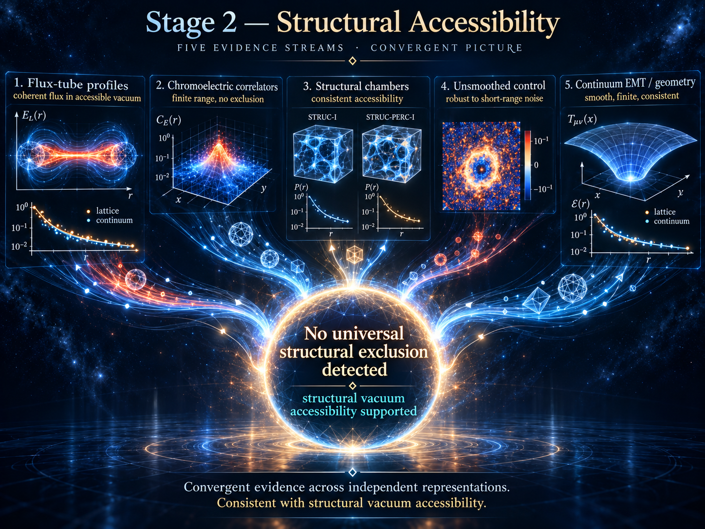
• Flux-tube profiles. Connected field profiles of the confining flux tube, with the vacuum contribution subtracted.
• Chromoelectric correlators. Finite range, no exclusion.
• Structural chambers. STRUC-I and STRUC-PERC-I readouts on the same profiles.
• Unsmoothed control. An independent dataset without smoothing, to check the architecture was not a smoothing artefact.
• Continuum EMT plus geometry variation. An energy–momentum-tensor representation, tested at three geometry radii.

The point is not that every branch said exactly the same thing. In fact, preserving different frozen verdicts is part of the strength. Some branches were calibration-sensitive. Some were refinement-indeterminate. EMT remained uncertainty-limited. Yet across the tested representations, no branch established a robust universal positive exclusion floor around the vacuum.

It is worth reading these verdicts the way they were written. They are a controlled negative result on one strong structural picture of the gap, set beside a positive spectral input that stays independent of the structural analysis. The non-detection of a floor is evidence about the structural side only. It says nothing about whether the spectrum is discrete, which the lattice anchors already settle numerically, and nothing about why.

6Stage 3: the spectrum did not come down with the wall

If no universal structural wall is established, does the spectral scale disappear with it? Stage 3 asked exactly that, and it was careful about how.

Figure 5 — Stage 3 — coexistence supported. Structural accessibility and spectral positivity coexist. Stage 3 retained two independent positive continuum scalar spectral scales in their native normalizations while leaving the structural analysis untouched. BRIDGE-III therefore supports coexistence — not a derivation of the mass gap, not a numerical identification between the two branches, and not a proof that the vacuum is a structural limit point.

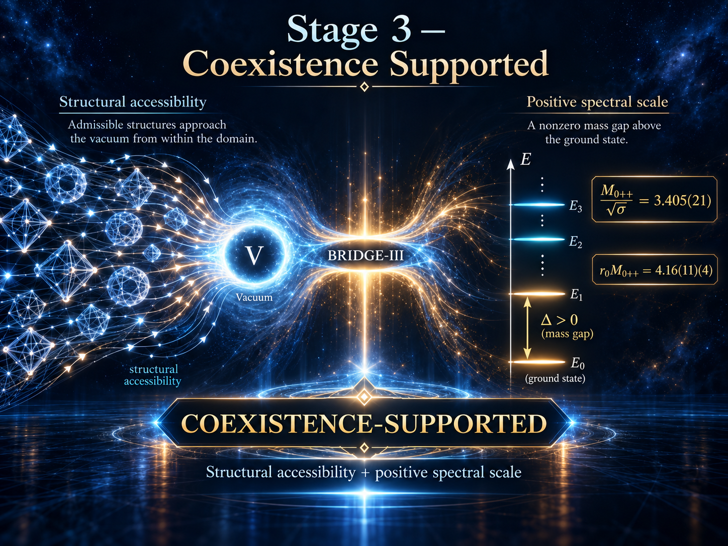
The two anchors stay in their native normalizations. They are not averaged and not converted into each other. And Stage 3 did not derive the spectral scale from the structural analysis. It did the opposite: it kept the two sides independent and asked whether they could coexist.

7The missing assumption

The mathematics behind the conceptual correction is elementary, but revealing. Write ε(X) for the excitation energy of a state X, and D_struct(X, V) for its structural distance from the vacuum.

A positive spectral gap alone does not imply a structural exclusion neighbourhood. But if ε is continuous at the vacuum, or locally satisfies a bound such as

then a positive gap does imply a structural exclusion radius: states with energy at least Δ cannot lie closer than δ = min{ r, (Δ/C)^1/α }. So the missing premise is a structure-to-spectrum continuity relation. The original wall picture had silently assumed exactly such a bridge.

The theorem’s value is diagnostic, not deep, and the manuscript says so. It locates a premise that had been doing all the work without ever being stated.

8Why this matters for Yang–Mills

This work does not solve the Clay problem. That boundary is a strength of the paper, not a weakness. The Clay problem asks for a construction of four-dimensional quantum Yang–Mills theory and a rigorous spectral gap, and nothing here provides either. The spectral inputs are numerical continuum extrapolations taken from published lattice calculations.

What the research does contribute is a constraint. Any account that claims

must now supply the missing continuity or Hölder bridge. The implication cannot simply be assumed. That is a real constraint on structural explanations of the gap, even for researchers who never use UNNS.

There is a converse. Suppose future work establishes the strong limit statement, a genuine physical sequence with

Then the discontinuity is no longer mysterious. It has to live in one of three places: in the structure-to-spectrum map Π, in the energy or support-edge functional on the space of spectral states, or in our choice of structural topology. The manuscript develops exactly these three readings. That gives the investigation something valuable: a sharply defined next problem instead of a vague philosophical conclusion.

If future work established a structural exclusion neighbourhood and independently justified an appropriate continuity or Hölder bridge, the two would be mutually consistent with the spectral gap. Structural exclusion by itself would not establish that continuity. Conversely, if a genuine physical sequence approached the vacuum structurally while the positive gap persisted, the required continuity of the structural-to-spectral-energy relation would have to fail somewhere.

Three things that are not the same thing

The work also keeps three ideas apart that are easily fused: confinement, the mass gap, and dynamical scale generation. The flux-tube data belong to confinement physics, and the analysis uses their vacuum-subtracted tails as structural probes. But a flux tube’s structural geometry is not automatically the spectral gap. Seeing flux tubes and concluding that their shape is the mass gap is exactly the shortcut the project declines to take.

9Monopoles, vortices, instantons and the rest

UNNS is not competing with center-vortex pictures, monopole and dual-superconductor pictures, instanton and caloron descriptions, or functional infrared approaches. Those programs ask what configurations or dynamics generate confinement and a dynamical scale.

This work asks a narrower and logically prior question: must structural proximity to the vacuum share the topology of spectral proximity?

Any microscopic mechanism could ultimately supply a continuous Π, a discontinuous Π, or a topology in which the relation behaves differently. A vortex account might yield one, a monopole-condensation account another; an instanton or caloron description might supply a structural coordinate from which spectral information is reconstructed; functional methods might define a spectral-state topology through Green’s functions. None is contradicted merely because structural and spectral nearness differ.

That makes the result mechanism-neutral, an important strength. The structural–spectral distinction works as a diagnostic layer that can be laid over several competing microscopic pictures, rather than as one more competitor among them.

10The methodological result matters too

The conclusions would mean little if they had been assembled after the fact. What separates this programme from a narrative reconstruction is its discipline.

• The Class C result was not allowed to overwrite Class B.
• The β = 6.71 crossing was preserved.
• CALIBRATION-SENSITIVE stayed calibration-sensitive.
• REFINEMENT-INDETERMINATE stayed indeterminate.
• EMT stayed uncertainty-limited, and thresholds were never moved.

Different chambers were not allowed to rescue one another. The programme gained not just another result, but a reusable epistemic discipline for keeping structural hypotheses falsifiable.

11The next problem is no longer the wall

The project leaves one central object behind.

Figure 6 — The next problem: construct Π. The next problem is no longer to find the wall, but to construct the structure-to-spectrum map. The synthesis identifies Π : 𝒮_UNNS → 𝒴_spec as the central open object: define the structural state space and metric, obtain paired structural–spectral data, determine the relevant spectral topology, and establish where continuity is preserved or fails. The programme remains mechanism-neutral with respect to center vortices, monopoles, instantons/calorons, and functional approaches.

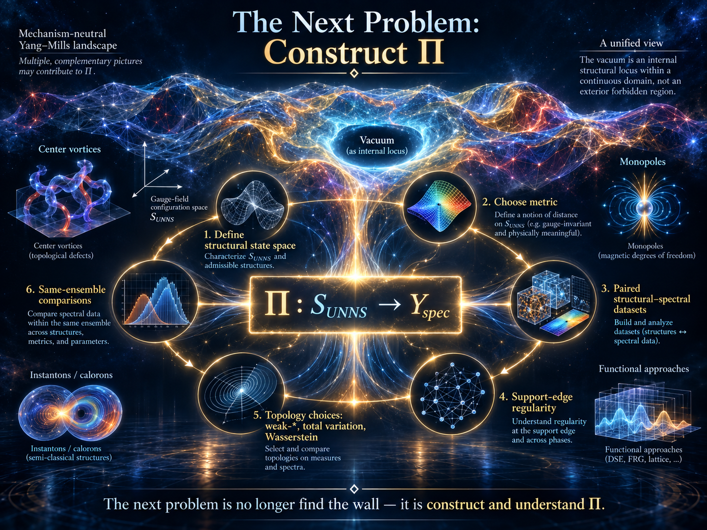
The new question is sharper than the old one: how does structural organization map into spectral data, and what topology makes that map continuous, discontinuous, or only partially regular? The concrete programme:

1. define the structural state space and a physically meaningful metric;
2. obtain paired structural–spectral data on the same ensembles;
3. construct finite-dimensional approximations to Π;
4. study support-edge regularity of the spectral functional;
5. compare weak-*, total-variation, Wasserstein and constrained topologies.

In other words, a search for a phenomenological boundary has become an identifiable structure-to-spectrum problem.

·What this changes for the UNNS view of the vacuum

The original UNNS picture of the vacuum was, roughly, an exterior one: admissible structure on one side, a forbidden region in between, and the vacuum beyond. The evidence did not support that geometry. The more successful reading treats the vacuum as an internal structural locus, a regime of the substrate that structure can approach, rather than a region sealed off behind an admissibility wall. The manuscript keeps this deliberately at the level of structural interpretation, not as a field-theory theorem.

It matters beyond Yang–Mills. An apparently discrete physical observable does not require the underlying structural substrate to be discretely partitioned in the same way. A continuous, internally approachable structural domain can support discrete spectral sectors, provided the map between structural organization and observable output is topologically non-trivial. That fits the broader UNNS principle that observable laws need not be primitive properties of the substrate: they may be stable outputs of a deeper organization.

The same statement is not specific to gauge theory. Whenever two layers of description coexist, microscopic structure and observable spectrum, geometry and eigenvalues, network organization and modes, the nearness checklist applies: before claiming that proximity in one space implies proximity in the other, say which topology is meant, and say why it should transfer.

The hierarchy of gains

What we are not claiming

The conceptual gain

We began by asking whether the Yang–Mills vacuum was protected by a wall. The evidence did not establish one. But the failure of that picture exposed something more fundamental: structure and spectrum are not obliged to approach the vacuum in the same way.

The gap may belong to the spectrum without appearing as a literal hole in structural space. The next task is therefore no longer to search harder for the wall.

What structure can approach and what the spectrum permits are different questions.