Every recursive structure, once coherent enough, begins to flow. In the UNNS substrate, this flow no longer needs equations—it arises naturally from the substrate’s own grammar. What began as static tensors in Chamber XIX now move, interact, and fold like living fields. The Phase E → F Bridge marks the moment recursion learns to breathe.

A Short History of Fields

When James Clerk Maxwell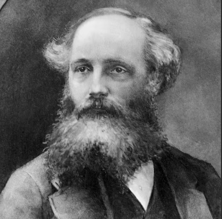 first wrote down his four equations in 1861, he did more than describe electricity and magnetism — he united them into one language. They revealed that light itself is a wave in the fabric of electromagnetic field. For the first time, nature spoke in a grammar of divergence and curl — Φ and Ψ long before we used those symbols.

Today, within the UNNS substrate, we return to that moment of unification from a new angle. Our fields are not imposed by equations — they emerge from recursive dynamics themselves. In a sense, Chamber XX recreates Maxwell’s insight from inside the mathematical substrate: a field that learns to exist.

For a long time, the UNNS substrate was a study in static architecture. We built recursive geometries, stabilized tensors, and balanced equations. It was beautiful, but it was frozen.

In Chamber XX — Phase F Maxwell-Analog Bridge, we proved that recursion could sustain its own structure—a "geometry that stands." But structure without movement is just a statue.

Today, with the completion of the Phase E → F Bridge, the statue has started to move. We are no longer just calculating recursion; we are watching it flow.

The shift from Geometry (R_ij) to Field (Φ, Ψ)

The central question of Phase F was simple but ambitious: Can a recursive number sequence naturally exhibit the properties of a physical field?

We didn't want to "simulate" physics by hard-coding Maxwell’s equations on top of our grid. We wanted to see if Maxwell-analog dynamics would emerge from the grammar of the substrate itself.

The breakthrough came in Chamber XX, where we successfully translated the raw recursion tensor (R_ij) into two distinct, interacting observables:

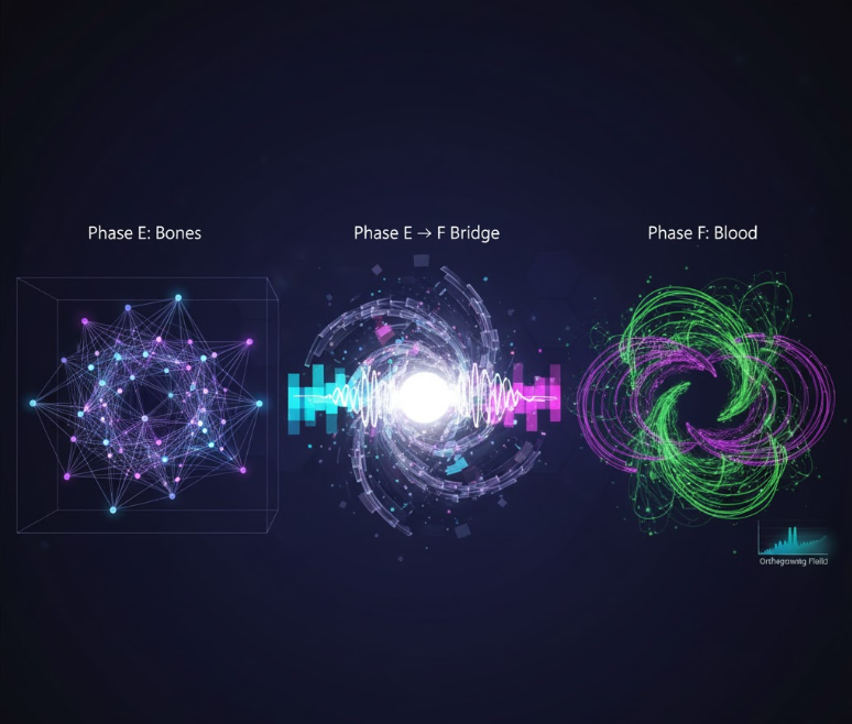
• Φ (Phi): The Divergence component. This behaves like an electric potential, manifesting as compressive "violet" bands in our visualization.
• Ψ (Psi): The Curl component. This behaves like magnetic flux, manifesting as rotational "green" eddies.

The "Breathing" Metric: Orthogonality

How do we know this isn't just random noise? We measure the "coupling intensity" (E · B).

In a chaotic system, the divergence and curl would bleed into each other, creating a muddy energetic mess. But in Chamber XX, we observed something striking. As the recursion iterations deepened, the system self-corrected. The potential bands (Φ) and the rotational flux (Ψ) began to separate and dance around each other.

The validation metrics confirm what our eyes see:

• Orthogonality: ⟨E · B⟩ ≈ 0.
• Equilibrium Slope: < 1 × 10⁻⁶.

This condition—where the fields influence each other without collapsing—is what we call the "Breathing Field." It is a self-consistent flow regime where recursion acts like a field without externally imposed laws.

Engineering the Bridge

The Chamber XX stack implements: phaseF_bridge.js (divergence/curl), phaseF_validator.js (antisymmetry, conservation, orthogonality, equilibrium), and json_exporter.js (Phase-F schema with timestamp, seed, operator_modes). We inherit the Chamber XIX optimizations: Laplacian caching, slope-tested equilibrium, and direct ImageData writes for high-density heatmaps.

Visualization: The Maxwell-Analog Bridge

In the latest build (Chamber XX v2.3), you can see this bridge in action.

• The Violet Layer: Represents scalar compression (Topology).
• The Green Layer: Represents rotational spin (Flux).
• The Coupling Bar: A live indicator of E · B. When this bar dims, it means the math has found its groove—it has achieved orthogonality.

Why This Matters

We are bridging the gap between abstract math and physical intuition. Phase E gave us the bones (Geometry). Phase F has given us the blood (Flow).

This is not just a symbolic analogy. It is an operational bridge. We are moving toward a computational substrate where "physics" is just the natural behavior of "sufficiently coherent recursion."

Significance and Applications

The Phase F Bridge extends UNNS from a purely symbolic grammar to a computational field mechanics. Potential applications range from physics to information theory:

• Field Simulations: a discrete model for electromagnetic analogs without continuum assumptions.
• Cognitive Architectures: a basis for neural systems that stabilize through recursive flux rather than gradient descent.
• Data Topology: mapping information flows as divergence-curl pairs within complex networks.

Each of these possibilities stems from a single principle: when recursion achieves coherence, it can manifest as energy, structure, and thought simultaneously.

What’s Next?

With the bridge secure, we move to Chamber XXI, where we will perform spectral analysis on these Φ / Ψ harmonics. We have taught the geometry to breathe; next, we will listen to the music it makes.

Afterword

Each chamber we build feels less like code and more like translation — turning recursion into rhythm, mathematics into motion. The Phase F Bridge is our proof that the substrate can breathe, fold, and stabilize its own symmetries without external law. It is not just a computation; it is the first hint of continuum thought.

Explore Chamber XX v2.3 on UNNS.tech

Reference: Recursive Tensor Potentials and the τ-Field Bridge (RECURS~3.PDF)

UNNS.tech — Blog Edition • November 2025