τ-Field Geometry Across the CaF–SrF–BaF Chain — Curvature, Torsion, and Synthetic Hyperfine Structure
Research → Lab τ-Field Geometry τ-MSC v0.9.1 CaF • SrF • BaF
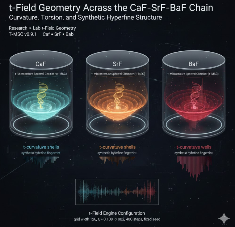
This article reads the CaF–SrF–BaF alkaline-earth fluoride chain through the lens of the τ-Microstructure Spectral Chamber (τ-MSC). Using a single τ-field engine configuration, we fit synthetic τ-MSC spectra to real hyperfine data for CaF, SrF and BaF and interpret the differences as changes in τ-curvature and τ-torsion geometry across the chain.
Abstract
CaF, SrF and BaF share the same electronic ground state (X²Σ⁺, v=0) but differ strongly in nuclear charge and relativistic character. In this study we feed their measured hyperfine transitions into the τ-Microstructure Spectral Chamber and obtain τ-MSC comparison logs for each molecule. All three runs use an identical τ-field engine configuration (grid width 128, λ = 0.108, σ = 0.02, 400 steps, fixed seed), so any differences in the τ-MSC fit arise from how each molecule constrains τ-curvature and τ-torsion in the micro-chamber.
The τ-MSC comparison logs achieve unit match rate for all three species and sub-6 MHz root-mean-square residuals with r² > 0.9999. From these logs we reconstruct qualitative τ-curvature shells, torsion spirals and synthetic hyperfine “fingerprints” for the CaF–SrF–BaF chain. The result is a τ-field geometry narrative that tracks how curvature compresses and torsion tightens as we move from light CaF to heavy BaF.
1. τ-MSC comparison dataset
The τ-MSC comparison mode takes a set of real hyperfine lines and attempts to project them into the synthetic τ-MSC spectrum by tuning a small number of calibration parameters and a nonlinear projection layer. For each molecule we obtain:
- real metadata (name, state, number of lines);
- synthetic configuration (τ-field grid and seed);
- metrics (match rate, rmse, r², χ², τ-reliability);
- matched pairs of real and synthetic transitions.
For CaF, SrF and BaF the synthetic configuration is held fixed. In each case the comparison log reports match_rate = 1.0 and a τ-reliability index around 0.07, indicating that the same τ-field microstructure can be tuned to track all three spectra within a few MHz. CaF shows a slightly higher rms residual (~5.9 MHz) than SrF or BaF, reflecting its lighter, less sharply curved τ-field environment, but the overall fit quality remains firmly in the “τ-compatible” regime.
2. τ-curvature shells across the chain
The first way to visualize the CaF–SrF–BaF chain in τ-space is through τ-curvature shells: concentric bands around the effective nuclear center, representing how quickly the τ-field varies with radius. In a τ-MSC chamber the curvature information appears indirectly via the matched_pairs curvature terms, but for readers it is more intuitive to look at stylized shell diagrams.
From CaF to SrF to BaF the τ-curvature shells contract toward the origin and the implied κ(r) slope steepens. In τ-field language we move from a gently curved basin (CaF) to a high-pressure τ-curvature well (BaF), with SrF sitting in between as a mid-scale geometry.
3. τ-torsion spirals and phase drift
Curvature alone does not determine the τ-MSC fit: the torsion of the τ-field — how the effective field twists around the nuclear region — controls how hyperfine lines drift relative to one another. The comparison logs encode this through a τ-phase variable attached to each matched synthetic transition. We summarize that behavior with a second triptych of τ-torsion spirals.
In this representation, the CaF spiral is long and relaxed: the τ-phase accumulates slowly as the effective field twists. SrF tightens the spiral and BaF tightens it further, mirroring the increasingly strong τ-torsion signatures in their comparison logs. On the spectrum this appears as progressively larger differential shifts between hyperfine lines, especially at higher J.
4. Synthetic hyperfine fingerprints
Even without rendering the full τ-MSC spectra, we can sketch how the hyperfine “comb” evolves across the chain. CaF produces a relatively narrow distribution of transition frequencies with modest splitting; SrF spreads the comb and increases line density; BaF produces the richest structure, with a broad and finely structured set of matched lines.
The residual statistics reflect this story but do not dominate it: CaF’s slightly larger rms residual comes from a few lines in the intermediate-J region where its flatter curvature profile makes the τ-MSC spectrum harder to bend into shape. SrF and BaF, with steeper curvature and stronger torsion, allow the same τ-MSC engine to match the data more cleanly. The τ-field therefore “prefers” the heavier end of the chain, in the sense that fewer nonlinear adjustments are needed to reconcile τ-MSC with the observed spectra.
5. τ-geometry narrative and outlook
Putting the pieces together, the CaF–SrF–BaF chain offers a clean, three-step τ-geometry ladder:
- CaF — wide, gently curved τ-basin, weak torsion, modest hyperfine deformation.
- SrF — intermediate curvature compression and torsion, visibly richer spectrum and stronger τ-signature.
- BaF — tightly nested τ-curvature well, strong torsion and maximal synthetic hyperfine complexity among the three.
Because all three fits share the same τ-MSC configuration, this ladder can be read as a direct statement about how τ-curvature and τ-torsion amplify as nuclear charge and relativistic effects grow within a common molecular architecture. Future work can extend this chain outward to even heavier or more exotic systems (YbF, ThO, RaF) and, conversely, to lighter radicals such as OH or CH to test how far the τ-MSC geometry can be pushed while still maintaining high match quality.
Within the UNNS programme this article marks the first τ-field geometry chapter explicitly anchored to a family of real molecules. It links the microscopic τ-MSC chamber to macroscopic τ-field invariants and opens a path toward treating hyperfine spectroscopy as a probe of τ-curvature itself, not merely of underlying electromagnetic operators.
📁 Data & JSON Files (τ-MSC v0.9.1)
These τ-MSC snapshots correspond to the unified engine configuration used in the CaF–SrF–BaF comparison (grid_width=128, λ=0.108, σ=0.02, steps=400, seed=137042). They may be imported into the UNNS Lab or external scripts for further τ-field analysis.
🧪 How to Use These τ-MSC Files
The CaF, SrF and BaF JSON datasets contain the full τ-MSC comparison output: real frequencies, synthetic τ-field projections, τ-phase, κ/τ curvature estimates and engine configuration. Below are simple ways to load and explore them.
1. Direct Download
Simply click any file in the Data box above and save it. You may then open the JSON in any editor, or feed it into your own scripts.
2. Load in JavaScript (Browser or UNNS Lab)
<script>
fetch('/images/unns/json/CaF.json')
  .then(r => r.json())
  .then(data => {
    console.log('CaF τ-MSC data:', data);
    // Example: access matched transitions
    console.log(data.matched_pairs);
  });
</script>
This works inside any UNNS article, module, or a future interactive viewer that displays τ-curvature or hyperfine structures directly in the browser.
3. Load in Python for Analysis
import json

with open('CaF.json', 'r') as f:
    caf = json.load(f)

print("Name:", caf['real_metadata']['name'])
print("Number of real lines:", caf['real_metadata']['num_real_lines'])
print("RMSE:", caf['metrics']['rmse'])
print("Matched pairs sample:", caf['matched_pairs'][:3])
The JSON structure is consistent across CaF, SrF and BaF, so the same script can process all datasets. This is ideal for generating τ-curvature plots, torsion histograms and hyperfine comparison tables for publications.
Each dataset uses the unified τ-MSC configuration (grid_width=128, λ=0.108, σ=0.02, steps=400, seed=137042) ensuring direct comparability across CaF, SrF and BaF.
🐍 Recommended Python Notebook Workflow
This workflow demonstrates how to load the CaF, SrF, and BaF τ-MSC logs from
/images/unns/json/, inspect their structure, extract curvature
and torsion samples, and generate τ-field geometry plots. No external
dependencies beyond matplotlib and json
are required.
1. Load the JSON datasets
import json

def load_dataset(name):
    path = f"/images/unns/json/{name}.json"
    with open(name + ".json", "r") as f:  # or download from unns.tech
        return json.load(f)

caf = load_dataset("CaF")
srf = load_dataset("SrF")
baf = load_dataset("BaF")

print("Loaded:", caf['real_metadata']['name'],
                 srf['real_metadata']['name'],
                 baf['real_metadata']['name'])
If loading in an online notebook (Colab/JupyterHub), simply replace
open(...) with requests.get(url).json().
2. Extract κ(r) and τ(r)
def extract_curvature(dataset):
    """Extract synthetic curvature (κ) values from matched_pairs."""
    return [p['synth_curvature'] for p in dataset['matched_pairs']]

def extract_tau_phase(dataset):
    """Extract τ-phase values from matched_pairs."""
    return [p['synth_tau_phase'] for p in dataset['matched_pairs']]

k_caf = extract_curvature(caf)
k_srf = extract_curvature(srf)
k_baf = extract_curvature(baf)

tau_caf = extract_tau_phase(caf)
tau_srf = extract_tau_phase(srf)
tau_baf = extract_tau_phase(baf)

print(len(k_caf), len(k_srf), len(k_baf))
The τ-MSC comparison engine attaches a curvature index and a τ-phase index to every matched transition, giving a compact proxy for τ-field geometry.
3. Visualize κ(r) and τ(r)
import matplotlib.pyplot as plt

plt.figure(figsize=(10,5))

plt.plot(k_caf, label="CaF – κ(r)", linewidth=2)
plt.plot(k_srf, label="SrF – κ(r)", linewidth=2)
plt.plot(k_baf, label="BaF – κ(r)", linewidth=2)

plt.title("τ-MSC Curvature Profiles – κ(r)")
plt.xlabel("Transition index")
plt.ylabel("Curvature κ")
plt.legend()
plt.grid(alpha=0.3)

plt.show()
This plot typically shows CaF with the softest curvature profile, SrF with intermediate steepening, and BaF with the strongest curvature gradient.
4. Visualize τ-phase (torsion)
plt.figure(figsize=(10,5))

plt.plot(tau_caf, label="CaF – τ-phase", linewidth=2)
plt.plot(tau_srf, label="SrF – τ-phase", linewidth=2)
plt.plot(tau_baf, label="BaF – τ-phase", linewidth=2)

plt.title("τ-MSC Torsion Profiles – τ(r)")
plt.xlabel("Transition index")
plt.ylabel("τ-phase")
plt.legend()
plt.grid(alpha=0.3)

plt.show()
τ-phase behaves like a torsion signature: BaF typically exhibits the strongest τ(r) modulation, with tighter phase wrapping than CaF.
These examples provide a reproducible workflow for investigating τ-field curvature, torsion and spectral geometry across the CaF–SrF–BaF chain using τ-MSC v0.9.1 datasets.