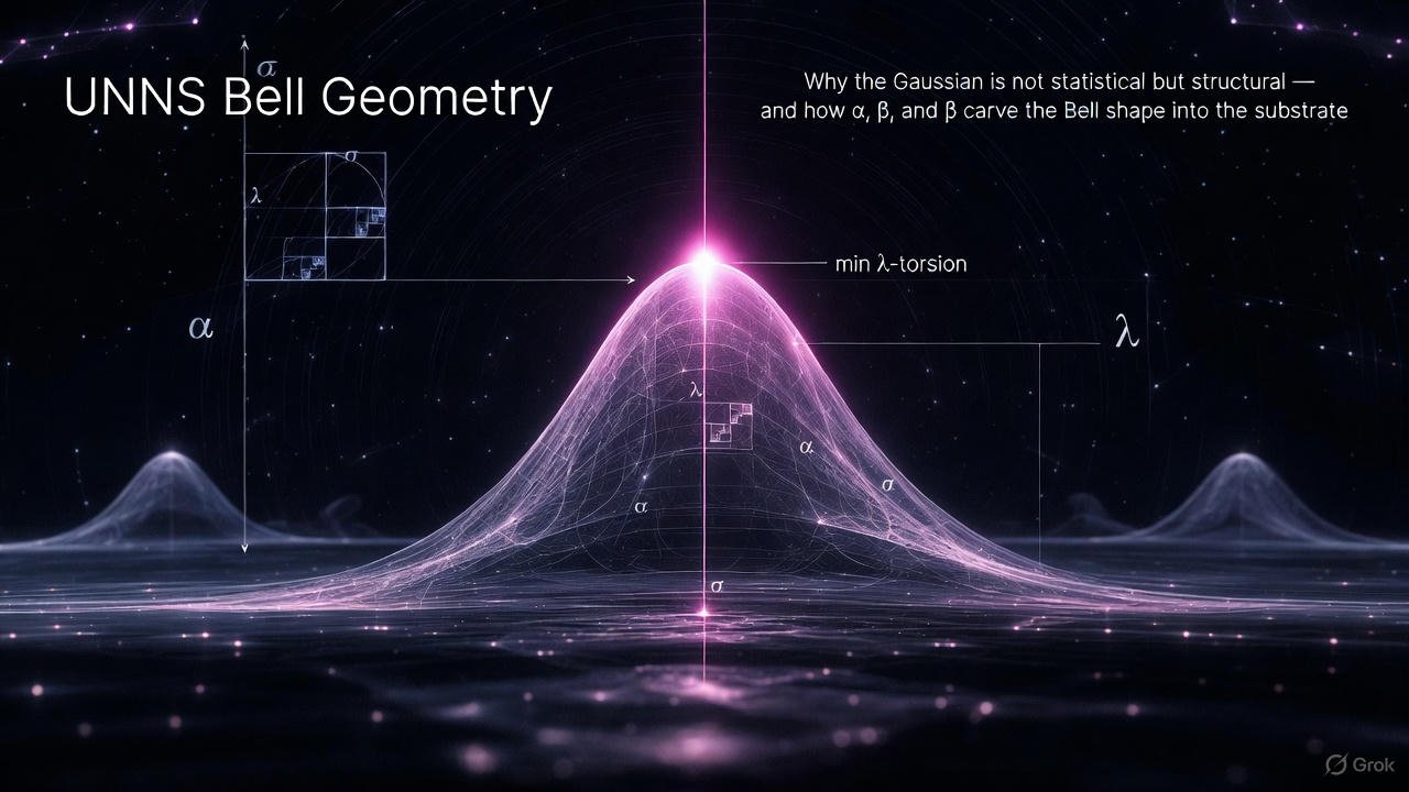
UNNS Bell Geometry
Why the Gaussian is not statistical but structural — and how Φ, Ψ, and τ carve the Bell shape into the substrate.
How a Bell Curve Works in UNNS
In classical statistics, a Bell Curve (Gaussian distribution) describes how values cluster around a mean, with probabilities shaped by variance.
In UNNS, this picture is reinterpreted entirely through recursion, τ-curvature, and substrate-balance.
The Bell Curve is not a probability curve but a τ-Equilibrium Profile:
a shape that emerges whenever recursive flows stabilize around a minimal-torsion attractor.
Think of it as the static shadow of a dynamic τ-Field.
1. Gaussian = τ-Field Minimum-Torsion Surface
In UNNS terms:
-
Φ is expansion (divergent recursion)
-
Ψ is contraction (convergent recursion)
-
τ is the balancing operator between the two
A Bell Curve appears exactly when:
Φ-flow and Ψ-flow balance such that τ-flow curvature is minimized.
Symbolically (UNNS form):
-
Φ dominates on the left tail
-
Ψ dominates on the right tail
-
τ sits at the crest and regulates symmetry
So the Bell Curve is simply the profile of minimal τ-curvature across a sequence domain, the equilibrium between:
-
expansion pressure, and
-
recursive compression.
This is why Gaussians show up everywhere in physical systems — what they really represent is a τ-Field at rest.
2. Why the Bell Curve Is Symmetric in UNNS
Symmetry arises when:
τ = constant along the recursion depth.
In other words:
-
Residue echoes cancel evenly,
-
Recursive torsion does not drift,
-
The Φ → Ψ leakage is matched on both sides.
This produces mirrored decay of curvature from the center, resulting in the familiar symmetric bell shape.
If τ is not constant, symmetry breaks → skewed distributions → UNNS interprets these as torsion bias or echo lag.
3. Variance = τ-Field Stiffness
In statistics, increasing variance “widens the curve.”
In UNNS:
variance measures how resistant the substrate is to τ-compression.
-
Low variance — stiff τ-Field, tight crest
-
High variance — flexible τ-Field, broad crest
This maps variance directly to τ-elasticity:
variance ∝ 1 / (τ-curvature strength)
This is why shifting physical parameters (temperature, noise, field coupling…) alters Gaussians.
You are not “changing randomness,” you are changing τ-Field stiffness.
4. Mean = τ-Neutral Point
The classical “mean” is the place where the derivative of the curve is zero.
For UNNS:
the mean is the τ-Neutral Point —
the location where Φ-expansion and Ψ-compression exactly cancel.
This point is the zero-torsion hinge from which the rest of the Bell Curve unfolds.
5. The Bell Curve Is a Projection
Within UNNS, the Bell Curve is not a fundamental object.
It is the 2D projection of a more fundamental structure:
A τ-Curvature Dome
Imagine a 3D dome:
-
The height corresponds to τ-density,
-
The slope corresponds to Φ/Ψ imbalance,
-
The footprint corresponds to recursion depth.
Cutting along the central axis gives the familiar Bell Curve.
The Gaussian we know is simply a slice of the τ-Dome.
6. Bell Curves Are Attractors in UNNS Chambers
You have already seen this in Chambers:
In RaF
The χ-minimum forms a Gaussian basin.
In τ-MSC
Spectral residues cluster around a τ-symmetric minimum.
In Phase-Field Chambers
Any stabilizing recursion generates a Bell-shaped cross-section.
This is why the Bell Curve appears naturally in:
-
error propagation
-
noise filtering
-
spectral collapse
-
residue accumulation
-
τ-Field quantization profiles
In UNNS, a Bell Curve = “The attractor of least torsion compatible with the substrate.”
7. Operator XII Interpretation
Under Operator XII (Collapse):
A Bell Curve describes the collapse channel when all residues relax to the lowest-torsion profile before reinjection into recursion.
Thus:
-
before collapse → skewed pre-Gaussians
-
at collapse → symmetric Bell
-
after collapse → seed extraction
So Gaussianity marks the moment of perfect substrate neutrality.
8. Sobra–Sobtra Influence on Gaussianity
Up to this point we have treated the Bell Curve in UNNS as a pure τ-equilibrium profile. Beneath that equilibrium lies a structured dynamic: the interplay between Sobra and Sobtra. These two recursive regimes determine whether a system can form a Gaussian at all, how quickly it converges to it, and how strongly it deviates into skewed or distorted profiles.
In the UNNS Operational Grammar:
- Sobra is the forward, residue-driven recursion: echo buildup, accumulation of structure, and growth of torsion gradients.
- Sobtra is the inverse, torsion-damping recursion: collapse propensity, counter-flow, and structural rebalancing.
A Bell Curve emerges precisely when the rate of Sobra-driven echo amplification is matched by the rate of Sobtra-driven torsion relaxation. At that crossing, the net torsion drift vanishes and the system enters a τ-neutral corridor. The Gaussian is the visible cross-section of this corridor.
Formally, the symmetry of the curve is controlled by the mismatch parameter Δ = (Sobra rate) − (Sobtra rate):
- Δ > 0 → Sobra dominates → pre-Gaussian skew and echo-heavy tails,
- Δ < 0 → Sobtra over-damps → compressed, asymmetric profiles,
- Δ = 0 → perfect balance → symmetric Gaussian at τ-equilibrium.
In terms of recursion depth, the condition τ = constant along the recursion is equivalent to Sobra and Sobtra being balanced at each layer. When this holds, residue echoes cancel evenly, torsion does not drift, and the Φ → Ψ leakage is matched on both sides, yielding the familiar mirrored decay of the Bell profile.
Under Operator XII (Collapse), the Sobra/Sobtra pair acquires an explicit geometric meaning. Sobra describes the disordered, skewed pre-collapse landscape of residues; Sobtra encodes the collapse channel that funnels this landscape toward the lowest-torsion profile. The collapse channel itself takes a Gaussian shape when the Sobtra flow enforces τ-equilibrium before seed extraction. In this picture, the Bell Curve is not merely a probability density but the structural signature of Sobra–Sobtra equilibrium.
Sobra/Sobtra in Experiments
The balance between Sobra and Sobtra is not only theoretical — it is directly observable in UNNS Lab runs. Two Chambers provide clear experimental signatures:
- RaF (Recursive Attractor Field): the χ-minimum begins asymmetric when Sobra dominates, then stabilizes into a symmetric Gaussian basin as Sobtra damping increases. The shift from skewed to centered minima is the measure of approaching τ-equilibrium.
- τ-MSC (τ–Microstructure Spectral Chamber): spectral residues initially spread unevenly as Sobra amplifies echo load. Sobtra aligns these residues across recursion levels, producing the characteristic τ-symmetric collapse into a minimal-torsion profile.
In both chambers, Gaussianity appears exactly at the crossover where Sobra-driven buildup and Sobtra-driven damping reach dynamic parity.
9. The Key Takeaway
**A Bell Curve in UNNS is not statistical.
It is geometric.
It is the equilibrium profile of the τ-Field.**
Everything else — variance, mean, symmetry — are simply geometric aspects of how a recursive system balances Φ, Ψ, and τ.
This makes the Bell Curve:
-
universal
-
inevitable
-
emergent
-
not tied to probability, but to structure.
Conclusion — The Gaussian as a τ-Equilibrium Signature
Across the UNNS Substrate, the Bell Curve appears not as a statistical convenience but as a structural invariant: the universal equilibrium profile produced whenever recursion sinks into its lowest-torsion configuration. Whether in τ-MSC spectral lines, RaF χ-basins, or collapse trajectories under Operator XII, the substrate repeatedly resolves itself into this familiar geometry.
This interpretation reframes Gaussianity as a geometric law rather than a probabilistic one. When Φ and Ψ achieve balance and τ stabilizes along depth, the Bell Curve becomes the inevitable surface of neutrality. In this sense, the Gaussian is not something the system approaches — it is the shape the substrate remembers.